- Published on
Transformer Architecture Explained
- Authors

- Name
- Trong Nguyen
As this blog will focus mainly on topics related to machine learning (and especially deep learning), I decided to write about the Transformer in this first post. This architecture, introduced in 2017 by Google researchers, is considered the backbone of modern NLP models (like GPT and BERT). Understanding its fundamentals is essential for exploring the world of Large Language Models.
TL;DR
- Before Transformer, models like RNNs processed tokens one by one, which made long-range dependencies hard to learn
- Transformer removed recurrence entirely, instead every token can directly look at every other token
- This is done through attention (self-attention and cross-attention) using Query, Key, and Value (QKV)
- Multi-head attention lets the model learn different types of relationships at the same time
- The model is built from stacked encoder and decoder blocks (attention + feed-forward layers)
- The encoder builds contextual representations of the input, while the decoder uses them to generate output token by token
- This architecture is the foundation of most modern AI models (e.g. GPT, BERT)
Sequential Data
In machine learning, we typically work with two input types: spatial and sequential data. Face recognition from an image and sentiment classification from a phrase are examples of spatial data, where the image or phrase provides the complete context needed for an output. However, many situations involve a temporal factor, for instance, speech transcription where voice is a series of frames, or action recognition from a sequence of images. Interestingly, these categories are not static: a single image can be treated as time-series data (like a sequence of scanned pixels), while sequential frames can be stacked into a single spatial input.
Combining sequential data into a single input presents several challenges. Without compression, the resulting data instances can become quite large, requiring significant computational resources. Conversely, compression often makes the information lossy. Such combinations can also weaken temporal relationships, reducing processing efficiency. To address this, many traditional methods handle sequential data by processing elements one by one.
To keep our focus consistent with the blog's theme, the remaining content will concentrate on Natural Language Processing (NLP), where sequential data corresponds to a sequence of tokens. If you are not familiar with the term token, thinking of it as a word is a good starting point (more details in the Tokenizing section).
Previous Models
Before the Transformer, NLP problems were typically handled by Recurrent Neural Networks (RNNs) such as Long Short-Term Memory (LSTM) and Gated Recurrent Units (GRU). These models process sequential data by iterating over each token, where the input for each step is the current token combined with the “memory” (hidden state) of everything seen so far. This mechanism has some key drawbacks:
Information loss: Memory is inherently lossy. The amount of information retained after processing tokens is often less than the tokens themselves, and this memory tends to fade as the sequence grows longer.
Limited context: In language, a token might have semantic relationships with others regardless of their distance. However, RNNs do not look at the entire input simultaneously for each token. As a result, they struggle to connect distant pieces of information.
As sequences grew longer, these limitations became significant bottlenecks. In essence, RNNs behave like reading a book only forward, never looking back, trying to remember the story while inevitably forgetting important details.
Transformer
The major improvement of Transformer comes from the ideology of dealing with the fundamental constraint of sequential computation by “eschewing recurrence and instead relying entirely on an attention mechanism to draw global dependencies between input and output”. Without using sequence-aligned RNNs or convolutions, the Transformer relies on its Multi-Head Attention mechanism to estimate representations of the input and output.
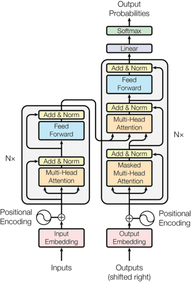
Transformer architecture (from the original paper “Attention is all you need”)
To be honest, the blocks on the left and right sides (and their connection) confused me initially. They are actually stacks of encoder layers (left) and decoder layers (right), which can be understood as follows:
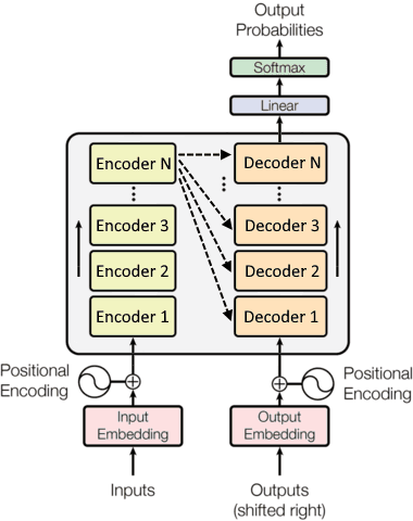
Alternate Transformer representation with stacks of layers (adapted from original figure)
Now let's break down the Transformer's components to understand them in detail.
Input Preparation
Neural networks only process numbers, while the typical input for NLP problems is text. A step to convert text to tensors is therefore mandatory. Let's use the phrase “The cats are sleeping while the dogs are running.” as input for demonstration.
Tokenizing
The first step of input preparation is tokenization, which separates the original text into a sequence of units called tokens. A token is a collection of characters with semantic meaning, which can be a whole word, a subword, or even punctuation. There are also predefined “special” tokens like [CLS] used in BERT or <|im_sep|> used in GPT-4o.
To be efficient, a tokenizer is trained on a large corpus to create a vocabulary of frequent tokens, where each is mapped to a unique ID. Thus, our input text becomes a vector of numbers. For example, using the GPT-2 tokenizer:
| The | cats | are | sleeping | while | the | dogs | are | running | . |
|---|---|---|---|---|---|---|---|---|---|
| 464 | 11875 | 389 | 11029 | 981 | 262 | 6844 | 389 | 2491 | 13 |
The input phrase is now represented as . Depending on letter case and position, the same word may be treated as different tokens (as with The and the). While sleeping and running are distinct tokens here, other tokenizers might split them differently (e.g., CodeLlama splits sleep and ing). More information about how tokenizers work can be found in this HuggingFace document.
Input Embedding
While the text is now numeric, it is still not quite ready for the Transformer. First, a single number (one-dimensional space) is not efficient enough to capture the complex semantic nuances of a token. Second, discrete values across a wide range (e.g., 30,000 for BERT) can lead to numerical instability issues, like vanishing/exploding gradients or activation saturation.
An embedding layer solves this by representing each token as a vector in a high-dimensional space (e.g., 768 dimensions in BERT). This layer acts like a lookup table which is actually a matrix where weights are learned during training. Its size is , where is the vocabulary size and is the embedding dimension (also called the hidden size).
Given a sequence of tokens, the “lookup” step using table mathematically is:
where the output embeddings contain a row vector of size for each of tokens, and is a matrix of one-hot vectors corresponding to the token IDs. In further illustrations, all graphs use specific values of , , and to give an idea about the tensor dimensions at each step.
In practice, these input embeddings are typically trained together with the whole Transformer, but they can also be initialized from pretrained models to leverage prior knowledge (especially with limited training data).
Positional Encoding
Since the Transformer lacks recurrence or convolution, it has no inherent sense of where each token sits in a sequence. We therefore need to explicitly provide this positional information. The original paper uses sine and cosine functions of different frequencies to encode positions:
has the same dimensions as the token embeddings , so they can be added together. The value belongs to the range as even and odd positions are filled separately. In practice, the term is often computed as for better numerical precision. Note that is the maximum wavelength scale that controls how fast or slow the sine and cosine waves change across dimensions. That value is used practically in the paper and should not be confused with the example vocabulary size (also ) described above.
Unlike the trainable embedding layer, this positional encoding is a fixed function of the element's position. However, some newer models use trainable positional encodings as well.
Input Formation
The final Transformer input is computed by applying a dropout layer to the sum of the token embedding and positional embedding . The following graph illustrates the input formation step applied to a sequence of 10 tokens with a vocabulary size of . The maximum allowed length for the input sequence in this example is , but it can be significantly higher in modern LLMs (usually known as the context window).

Input processing for a sequence of 10 tokens before feeding to Transformer
Encoder
An encoder is a stack of identical layers (6 in the original paper), where the output of one layer serves as the input for the next. As data passes through these layers, the representations become increasingly abstract and context-aware. By the end of the encoder pipeline, each token's embedding has been “enriched” with information from the others across the entire sequence.
Encoder Layer
The following graph illustrates the computation within an encoder layer, which is a stack of two residual connections (i.e. the processed result of an input is added back to that input) followed by layer normalization like .

Encoder layer as stack of two residual connections followed by layer normalization
Residual connections are crucial for training deep networks as they provide a “shortcut” for gradients to flow backward, mitigating the vanishing gradient problem. Layer normalization is used instead of batch normalization because it normalizes across the features of each token independently, making it more stable for varying sequence lengths. While both residual blocks use dropout with a ratio of 0.1, they differ in their use of multi-head attention and feed-forward layers as different implementations of .
Scaled Dot-Product Attention
The heart of the Transformer is the Attention mechanism. By considering the input as a series of tokens, the model needs a way to decide which other tokens are relevant to the one it is currently processing. This is achieved using three vectors derived from the input embeddings: (query), (key), and (value). According to my understanding, the three terms can be interpreted as follows:
- The query corresponds to the current token being processed
- The key represents all tokens in the sequence
- The value is the information contained within those tokens
The attention mechanism calculates the relevance, known as the attention score, by comparing the query (current token) with all keys (other tokens in the sequence) using a dot product, i.e. . This score is then scaled (by a factor of ) and normalized using softmax to create a probability distribution (or attention weights), which is then used to weight the values :
where is the dimension of keys. The factor prevents the dot products from growing too large, which would push softmax into saturation and cause near-zero gradients.
The following graph illustrates the computation of scaled dot-product attention with . The mask is optionally used to prevent attention from considering certain positions. For example, padding tokens should be ignored when processing batches of sequences with different lengths, or future tokens should not be attended to during the training stage of text generation models (i.e. prediction for the token depends only on the known output tokens before position ). The values corresponding to non-attending positions in an input tensor are replaced by a very small number ( in the following graph) to ensure the output softmax is almost 0.

Computation of scaled dot-product attention with optional mask
The number in the tensor dimensions is related to the number of heads in the following Multi-Head Attention mechanism.
Multi-Head Attention
This mechanism performs the above attention computation in parallel, i.e. multiple attention operations given the three inputs , , and . This allows the model to attend to information at different positions from different perspectives. For example, one head might focus on semantic meaning, while others focus on grammatical relationships or co-reference.
For each head, the inputs go through learned linear projections (i.e. representing them in a subspace corresponding to a meaningful perspective) before being fed into the scaled dot-product attention. Those heads are then concatenated and once again projected to produce the final value of the multi-head attention. The following figure shows a generic computational flow of 8-head attention.

Multi-head attention with 8 parallel heads and an optional mask
Feed-Forward Network
In each block of the encoder (and decoder), the attention is followed by a fully connected feed-forward network (FFN). This FFN is a stack of 2 linear transformations separated by a ReLU activation. These linear layers can be thought of as convolutions with kernel size 1. The input and output of the FFN have the same dimension , but the inner layer has dimensionality , as visualized in the next graph.

Position-wise feed-forward network which follows the attention part
What makes this “position-wise” is that the same FFN is applied to each token position separately and identically. While attention allows tokens to communicate with each other, the FFN allows the model to process the information gathered for each token individually, effectively “digesting” the contextual data.
Decoder
Similarly to the encoder, a decoder is also a stack of identical layers. As visualized in the alternative figure of the Transformer architecture, the inputs to a decoder block include the output of its predecessor and the output of the encoder.
Decoder Layer
The decoder layer is designed as a duplicate of the encoder layer with an additional sub-layer that performs multi-head attention over the embedded information output from the encoder part of the Transformer. The encoder's embedding plays the role of and , while the output of the previous decoder layer is used as . Masks are used in both attention mechanisms, in which the first one (in self-attention) is to prevent tokens from attending to subsequent positions while the second attention (cross-attention with encoder outputs) considers padding masks. This masking ensures that the prediction at position only depends on the information from positions before .

Decoder layer which is similar to encoder layer with an additional block of residual connections in the middle
Linear Classifier & Softmax
After the decoder stack produces a final vector for each position, we need to turn these numbers back into actual words. A linear layer projects the decoder output into a much larger vector with the size of the vocabulary ( in our example). The scores in that vector are then converted into probabilities via softmax, and the token with the highest probability is selected as the next token in the sequence.
Conclusion
The Transformer architecture represents a paradigm shift in how we approach sequence modeling. By replacing the sequential processing of RNNs with parallel attention mechanisms, it addresses the fundamental limitations of information loss and limited context that plagued earlier models. The key innovation, which is allowing each token to directly attend to all other tokens in the sequence, enables the model to capture long-range dependencies and complex relationships that were previously difficult or impossible to learn.
What makes the Transformer particularly powerful is its elegant composition of relatively simple components: scaled dot-product attention, multi-head attention for multiple perspectives, position-wise feed-forward networks for individual token processing, and residual connections with layer normalization for stable training. Together, these elements create a system that is both parallelizable (making it efficient to train on modern hardware) and expressive (capable of learning rich representations).
Since its introduction in 2017, the Transformer has become the foundation for virtually all state-of-the-art NLP models. GPT's decoder-only architecture powers modern chatbots and text generation systems. BERT's encoder-only design excels at understanding and classification tasks. More recent models like T5 and BART use both encoder and decoder stacks for translation and summarization. Beyond NLP, the attention mechanism has also been successfully adapted to computer vision (Vision Transformers), speech processing, and even protein structure prediction.
Understanding the Transformer is no longer optional but essential for anyone working in modern machine learning. As we continue to scale these models and apply them to new domains, the fundamental principles laid out in “Attention Is All You Need” remain as relevant as ever. This architecture has proven that sometimes the best solution is not to make our models remember better, but to give them the ability to look at everything at once and decide what matters.
Advanced Questions & Insights
Because attention is expensive.
Self-attention has an cost with respect to sequence length (as each token compares itself with every other token), which was simply not practical before modern GPUs/TPUs.
RNNs were a workaround:
- Process tokens sequentially
- Scale linearly with sequence length
- Trade performance for feasibility
Reality check: RNNs were not replaced because they were wrong, but because hardware finally caught up.
Because it removes the need to carry information step-by-step.
- In RNNs: information must pass through many steps → vanishing gradients
- In Transformer: any token can directly attend to any other token in one step
Result:
- Much better handling of long-range relationships
- More stable training
Key insight: Direct token-to-token access collapses the path length between any two positions from to .
Because attention is order-agnostic.
Without positional information, the model sees a sentence like a bag of words, ignoring order (e.g., “Alex buys pizza” vs. “pizza buys Alex” 😵💫).
Positional encoding:
- Injects sequence order into the model
- Becomes critical for long-context understanding
Interesting note: Relative positional encoding often generalizes better than absolute ones.
From the perspective of a search engine:
- Query = what I'm looking for
- Key = what each token offers
- Value = the actual information
Process:
- Match Query with Keys → relevance score
- Use that score to weight Values
Key insight: Attention is basically “search + weighted aggregation” dressed up in linear algebra.
It mostly learns statistical correlations, not true reasoning.
Attention maps sometimes look interpretable (e.g., aligning related words), but:
- Some heads clearly track meaningful relationships
- Many are noisy or redundant
Key insight: Interpretability is a side-effect, not the objective (it is optimized for prediction, not explanation).
In principle, a single head could learn diverse relationships.
In practice, multiple heads are used to:
- Capture different types of relationships simultaneously (syntax, semantics, position, etc.)
- Reduce the risk of collapsing everything into a single representation
But actually:
- Many heads end up doing almost nothing
- Heads can be pruned with minimal impact
Reality check: Multi-head attention is partly useful, partly redundancy for stability.
Because of quadratic scaling:
- Memory:
- Computation:
Every token attends to every other token → long contexts (e.g., 100k tokens) are extremely expensive.
That is why we see alternatives like:
- Sparse attention
- Linear attention
- or sidestep it entirely with retrieval (RAG)
Reality check: Many real-world systems use retrieval instead of actually solving long context.
(In my opinion), Transformer is closer to brute-force.
It does not compress information efficiently, instead it:
- Uses massive parameter counts → larger models can approximate more complex functions
- Relies on huge datasets → more data reduces overfitting
- Scales compute aggressively → training finds better minima in high-dimensional space
But (important) it works.
Blunt truth: Transformer models succeed less because they are theoretically optimal, and more because scaling them is incredibly effective.
Short answer: not in the way humans do, instead it:
- Simulates reasoning largely through pattern matching
- Performs well on structured tasks
- Breaks on edge cases requiring strict logic
Key insight: Transformer is extremely good at looking like it reasons.
That attention is the only thing that matters.
In reality, performance comes from the combination of:
- Attention
- Feed-forward layers (often most of the parameters)
- Training data
- Optimization tricks
Interesting note: Attention gets the spotlight, but feed-forward layers do a huge amount of the actual work.
Probably, but smoothly instead of suddenly.
We are already seeing pressure from:
- State space models (e.g., Mamba)
- Retrieval-based systems
- Hybrid architectures
But Transformer still dominates because of:
- Ecosystem maturity
- Proven scalability
- Strong tooling
Expectation: Transformer will get embedded into hybrid systems.